Introduction:
The purpose of this blog is to give an overview of
“Theoretical & Computational Fluid Mixing using Rotating Impeller”. Current Chemical & Bio-technical Process Industry widely used different types of Impellers according to their requirements which demands adequate & uniform concentration and temperature. The essential task of the mixers is to bring together two or more fluids and/or solids which are initially separated. Mixing could be accomplished either by rotating impellers or by jets of liquid. Mixing by rotating impellers is the point of interest for as of now for this blog. Liquid Jet Mixing explained
here. Also, check agitator design aspects
here.
McCabe rightly quoted “Many processing operations depend for their success on the effective agitation & mixing of fluids”. Desired mixing process could be Multiphase or Single phase, reacting or non-reacting, laminar or turbulent, Isothermal or Non-isothermal depending upon materials to be mixed and requirement. In most of processes mixing equipment is a simple batch reactor tank with an impeller mounted on a shaft and optionally can contain baffles, and other internals (spargers, coils and draft tubes). The optimum design of a such mixing equipment depends on the desired production rate, properties of the fluids/solids to be mixed, choice of tank and impeller geometry, rotational speed and location of fluid addition and removal. The typical configuration of a stirred tank is shown below in Figure. 1.
Figure. 1 Typical Configuration of a Stirred Tank
PART [I] Theoretical Background:
Introduction:
In general, mixing refers to any physical operation used to change a non-uniform system into a uniform one. It involves processes such as blending, dissolving, dispersion, suspension, emulsification, heat transfer and chemical reaction. The electric motor is used to rotate the shaft and impeller which transfers the momentum to the fluids by means of blades. The momentum transfer from blades to fluid is basically due to shearing and normal stresses. In earlier transfer mechanism, the momentum transfer is perpendicular to the flow direction. Whereas in later transfer mechanism the momentum transfer is parallel to the flow direction. Based on these two-momentum transfer mechanism, agitator classification can be made. The shearing stresses momentum transfer includes the rotating disc and cone type agitators and the normal stresses momentum transfer includes the paddle, propeller, and turbo mixer agitators. The momentum of the fluid gain from the impeller blades must be enough to carry material into the most parts of the tank. Therefore, with little understanding of flow types one can conclude that mixing is more effective in turbulent regime compare to laminar. This also can be understood by knowing phenomena’s which contributes mixing. The mixing in the tank is contributed mainly by two phenomena’s,
Distribution; in which materials are transported to all regions by advection i.e. bulk circulation currents and
Dispersion; in which the eddies (possessing kinetic energy) formed by continuous stirring breakup into smaller eddies. Some characteristics of distribution and dispersion are given below in Table. 1. Other than these two parameters, the third important parameter which plays a vital role is momentum transfer by molecular
Diffusion; here, mixing take place on a scale smaller than
komogorov scale .
Table. 1 Characteristics of different Mixing Phenomena’s
Impeller Types, Selection & Flow Field:
Impellers are classified conveniently according to the dominance of flow direction. However, due to baffles and other internals, flow patterns in most cases are mixed. Fig. 2 provides some different types of impellers used in industries. While selecting impellers some agitating fluid characteristics is essential to study, which are given below:
Characteristics for agitating fluids:
- Blending of two miscible or immiscible liquids.
- Dissolving solids in liquids.
- Dispersing a gas in a liquid as fine bubbles (e.g., oxygen from air in a suspension of microorganism for fermentation or for activated sludge treatment).
- Agitation of the fluid to increase heat transfer between the fluid and a coil or jacket.
- Suspension of fine solid particles in a liquid, such as in the catalytic hydrogenation of a liquid where solid catalyst and hydrogen bubbles are dispersed in the liquid.
- Dispersion of droplets of one im-miscible liquid in another (e.g., in some heterogeneous reaction process or liquid-liquid extraction).
Figure. 2 Impeller Types
Table. 2 Provides in brief classification of agitator types with their application, advantages & disadvantages. Also, Fig. 4 provides selection of an impeller based on viscosity of agitating fluid. However, the performance of a shape, size and no of blades of impeller usually difficult to predict which requires experimental or computational resources. Here comes the role of Computational Fluid Dynamics (CFD) to judge the performance of a given design. With robust CFD methodology it is easier to have a judgment on mixing characteristics.
Figure 3 Impeller Type Selection based on Fluid Viscosity
Table. 2 Classification of Agitator Types with their Application, Advantages & Disadvantages
Assessing & Optimizing Mixing:
According to industry requirement and with natural limitations by mixing fluid and agitator design, assessment and optimization is vital. In most of times mixing time and power required for mixing considered for the assessment & optimization by varying angle of shaft insertion in tank, angle of tip to end of a blade, no. of blades size of the blade etc.
As name suggest, it is time required to achieve desired homogenized/uniform solution. Experimentally, it can be measured by injecting tracer into the vessel and following concentration at a fixed point in the tank. Using CFD will be discussed in PART [III]
- Power Requirement for Mixing:
Electric powered motor is usually used to drive the impeller in the tank. Power requirement for mixing is essentially depending on resistance offered by the fluid to rotation of the impeller. However, fluid properties, required level of mixing, tank size, impeller type & size are also important. The power requirement per unit fluid volume ranges from 10 kW/m
3 for small tanks to 1~2 kW/m
3 for large tanks. For the power requirement calculation, it is always preferable to work with dimensionless numbers such as the impeller Reynolds number
(Re), Flow Number
(NQ) and the Power Number
(Np).
Essential Dimensionless Numbers in Mixing Tank Analysis:
Dimensional numbers are very helpful when dealing with fluid flow operations. Some desired numbers useful for optimum design of mixing equipment are given below:
- Impeller Reynolds Number (Re) : To characterize flow regime
- Power Number (Np): To calculate power consumed by the turbine
- Flow Number(NQ): To express pumping capacity
Q is volumetric flow rate (m
3/s), μ = fluid viscosity (Ns/m
2), N
i = Rotational speed of the stirrer (revolution per minute), P = Power (Watt), ρ = density of the mixing fluid (Kg/m
3), D
i = impeller diameter (m)
Also, there has been vast study carried out using these numbers to provide correlations to calculate mixing time and power requirement.
PART [II] CFD Aspects for Mixing Tank Analysis:
Introduction:
Computational Fluid Dynamics is very useful to assist in the design, optimisation and scale-up of mixing tanks. Still, there are some difficulties which have been countered by some approximation of the physical phenomena, such as turbulence model, rheological models for non-Newtonian fluids and impeller boundary conditions. The basic equations solved in a mixing calculation i.e. conservation of mass, momentum and energy can be found in a standard chemical engineering books. Fundamental CFD approach can be found in fundamental CFD books.
Representation of the Rotating Impeller:
Resolving rotating impeller-fluid is one of the complicated challenges faced by CFD developers. There are few strategies developed to counter the same, described in brief below:
(a) Use of a Momentum Source Term:
The momentum exchange between the impeller blades and the bulk fluid is resolved by empirical co-relation extracted experimentally. However, it is not fully predictive, reliable and implicit.
(b) Single & Multiple Frames of Reference (SRF & MRF):
SRF solves governing equations using single rotating frame only, whereas MRF solves rotating zone in rotating reference frame and stationary zone in stationary reference frame. Both approaches don’t count the impeller rotation, it is fixed in one position. Therefore, it can only predict the steady state flow field and does not account for transient impeller-baffle interactions. Using these two methods it is not possible to calculate the mixing time.
(c) Sliding Mesh Approach:
The Sliding Mesh Approach is the only method which can resolve transient impeller-baffle interaction and provides more accurate solution comparatively. However, the computational cost is more. The basic idea in Sliding Mesh Approach is to employ two grids one of which rotating in small angular steps with the impeller while the other is fixed to the tank. At each step the flow field is recalculated to take into account the new impeller position. Moving mesh is allowed to slide relative to stationary one and interpolation between two meshes is provided by the special cyclic boundary condition. This method allows us to calculate mixing time.
Turbulence Model Selection:
Most of industrial mixing tank problems involves turbulent flow. In turbulent flow regime, the dispersion plays an important role for mixing therefore it is preferable to utilized robust turbulence model. Large Eddy Simulation (LES) and Direct Numerical Methods (DNS) are not preferable to solve large industrial problems due to high computational cost, though they provide highly accurate solution. Therefore, approximated Reynolds Navier Stokes (RANS) two equation model such as k-epsilon & k-omega widely used to solve industrial problems involving turbulence.
For mixing tank problems, vortices and circulation occurred near impeller blades are the source for eddy formation and are vital for momentum transfer and hence for mixing. Therefore, resolving of such flow phenomena should be utmost priority while model selection. The standard k-epsilon & k-omega model has been criticised for poor performance with swirling or recirculating flow which occurs in mixing tank. To account recirculation and vortices, Curvature Correction (CC) modification has been added to the standard RANS models. Furthermore, modifications have been done to predict the onset of separation using Shear Stress Transport (SST) Model and Reattachment Modification (RM) model to account large separation zones. Overall, modified blend of SST-RM-CC model can provide better solution to encounter turbulence occurred in mixing tank. However, with all these modifications to standard two equation model dissipation rate is still underpredicted and turbulence is assumed to be isotropic.
To overcome these two problems Reynolds stress transport equations based “Explicit Algebraic Reynolds Stress Models” (EARSM) has been developed. More details about these models can be found in standard books such as Computational Methods for Fluid Dynamics by J. H. Ferziger or else ANSYS CFX theory manual.
From literature, it has been found that while most of turbulence models provides good predictions of the mean flow field. However, the accuracy of predictions of turbulence kinetic energy and its dissipation rate has generally been quite poor. However, SST-CC, SST-RM-CC and EARSM can be used accordingly for simulating mixing tank problem.
PART [III] Computational Fluid Mixing using Rotating Impeller; A Case Study using OpenFOAM
Introduction:
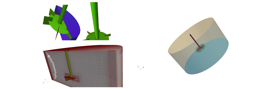
In this case study, CFD modelling methods have been applied to predict the fluid flow fields in a mixing tank. The aim of the study is to predict the mean velocity, mixing time, power required by the impeller. The geometry of the mixing tank consists of a cylindrical vessel with Rushton turbine and baffles. The cylinder is 1 meter long and 1 meter of radius (not standard) as shown in Fig. 4. The fluid in the tank is water only. For the analysis, open-source OpenFOAM CFD tool has been utilized which is widely recommended in scientific community due to its customization ability. Here, also, the base code has been modified to calculate the mixing time by adding scalar transport equation to the main source code. The study includes mesh generation, modelling approach and post processing. The turbulence model selection has already been discussed above in PART [II].
Figure 4. Mixing Vessel with Ruston Turbine
Mesh Generation:
For the analysis the meshing has been done using snappyHexMesh tool comes with OpenFOAM, which is purely 3D finite volume mesh generator supports hexahedra and split-hexahedra mesh. For the current analysis the volume cells restricted around ~100000 but practical industrial applications demand is multiple of it. Due to large variable gradients nearby blades and other rotating parts, the mesh is dense nearby the blades as shown in Fig. 5 and coarser away from it. Typically, using coarser mesh mean flow velocity can be predicted well but for turbulence parameter mesh resolution needs to be increased in step wise manner nearby the rotating regions. Here, the mesh nearby the rotating region is more than 45% accommodates volume less than 25 %. Finally, the grid independent study is must before jumping on to main simulation setup.
Figure 5. Generated Mesh for Mixing Tank
Numerical Methods:
The convective terms discretized using second order upwind scheme and temporal parameters using second order backward Euler scheme. Before using second order discretization schemes 1
st order schemes used for few iteration steps for the sake of stability.
K-Omega SST model has been selected for the current analysis due to its ability to work nicely with curvature/swirling flow along with Sliding Mesh Approach to represent rotating impeller. To resolve pressure-velocity coupling combination of PISO & SIMPLE i.e. PIMPLE algorithm has been selected.
Reducing Simulation Time:
In practice, it is possible to reduce the simulation time maintaining greater accuracy
. Different approaches for solving rotating impeller problems have already been discussed. The MRF method provides good predictions of the flow field, however it is not possible to calculate mixing time. Whereas Sliding Mesh Method provides all the information we need however, it has high computational cost. To reduce the simulation time following steps are preferable:
- Work with coarser Mesh using MRF Method for initial few iterations.
- Then apply the developed flow fields to fine mesh and run for few iterations using MRF method.
- Finally, switch to Sliding Mesh Method.
- If turbulence parameters are not converging then let the field be developed using laminar flow and then switch to turbulence model.
Results & Discussion:
Soon will be updated